1. The Soil-Water Interface: Infiltration Physics and Unsaturated Zone Mechanics
The terrestrial water cycle hinges upon a fundamental physical partition that occurs at the very surface of the Earth: the separation of incoming meteoric precipitation into surface overland flow and subsurface soil infiltration. The capacity of a landscape to absorb water governs flood frequency, agricultural productivity, contaminant transport, and the sustained replenishment of regional aquifers. This dynamic interface is governed by infiltration mechanics operating within the unsaturated (vadose) zone of the soil matrix.
Infiltration is defined as the downward entry of liquid water across the atmosphere-soil boundary into the soil profile. The rate at which soil can absorb water at any given moment is termed its infiltration capacity (f_p, expressed in mm/hr). When rainfall intensity (i) is less than infiltration capacity (i < f_p), all incoming water infiltrates into the soil, leaving the surface dry. However, when rainfall intensity surpasses infiltration capacity (i > f_p), surface depression storage fills, and the excess water begins flowing downslope as Hortonian overland flow (infiltration-excess overland flow).
The mechanics of infiltration are governed by two distinct physical forces: matric suction (capillary tension) and gravity. In dry soils, capillary forces generated by the surface tension of water menisci within narrow soil pores exert powerful negative matric potentials (matric suction heads, ψ < 0), pulling water molecules violently into the pore matrix. As infiltration proceeds, the soil pores fill with water, reducing the capillary suction gradient toward zero. Consequently, infiltration capacity exhibits a characteristic decaying exponential curve over time, initially high when the soil is dry and asymptotically declining toward a constant, steady-state minimum dictated purely by gravity and saturated hydraulic conductivity (K_sat).
To mathematically quantify this decay, Robert E. Horton formulated his classic empirical infiltration equation (1939): f(t) = f_c + (f_0 – f_c) · e^(-k·t), where f(t) is infiltration capacity at time t, f_0 is initial infiltration capacity, f_c is ultimate steady-state saturated capacity, and k is an empirical soil decay constant. In 1911, W.H. Green and G.A. Ampt developed a more physically rigorous, process-based formulation based on Darcy’s Law: f(t) = K_sat · [1 + (ψ_f · Δθ) / F(t)], where ψ_f is wetting front suction head, Δθ is moisture deficit, and F(t) is cumulative infiltrated water depth, capturing the physics of the sharp ‘wetting front’ that descends through the soil column.
💧 Hydraulic Law: Green-Ampt Infiltration Formulation
The Green-Ampt equation models infiltration as a piston-like wetting front descending through an unsaturated soil profile. Capillary suction dominates early water absorption, but as the saturated zone deepens, the hydraulic gradient approaches unity, and infiltration capacity asymptotically approaches saturated hydraulic conductivity (K_sat).
2. Subsurface Fluid Mechanics: Darcy’s Law and Aquifer Hydraulics
Once infiltrated water percolates past the plant rooting zone under the force of gravity (deep percolation), it transitions from the unsaturated vadose zone across the phreatic surface (the water table) into the saturated groundwater zone. In this subterranean realm, all pore spaces, lithological fractures, and voids are 100% filled with water under positive hydrostatic pressure (P > P_atm).
The foundational mathematical law governing fluid flow through porous media was empirically established by French engineer Henry Darcy in 1856 during his experiments on sand filters in Dijon. Darcy’s Law dictates that volumetric groundwater discharge (Q) through a porous medium is directly proportional to the cross-sectional area (A) perpendicular to flow and the hydraulic gradient (dh/dl), scaled by the hydraulic conductivity (K) of the geological medium: Q = -K · A · (dh / dl), or in specific discharge (Darcy flux, q = Q/A): q = -K · (dh / dl).
In Darcy’s formulation, the hydraulic head (h) represents total mechanical fluid energy per unit weight, combining elevation head (z, gravitational potential) and pressure head (P / [rho · g], porewater pressure): h = z + P / (rho · g). The negative sign signifies that groundwater always moves down the hydraulic gradient from regions of higher hydraulic head to regions of lower hydraulic head, regardless of physical elevation (e.g., groundwater can flow vertically upward if deep artesian pressure head exceeds the elevation drop).
Hydraulic conductivity (K) is a combined property of both the porous rock medium and the fluid: K = k_i · (rho · g / mu), where k_i is intrinsic permeability (dictated purely by grain size distribution, pore geometry, and tortuosity, measured in Darcies or m²), rho is fluid density, g is gravitational acceleration, and mu is dynamic viscosity. In natural geological formations, hydraulic conductivity spans an astounding fourteen orders of magnitude—ranging from 10^-2 m/s in clean gravels and karstic limestone conduits down to 10^-12 m/s in intact clays, unfractured shales, and crystalline granites.
| Geological Material | Hydraulic Conductivity (K, m/s) | Effective Porosity (ne, %) | Transmissivity Potential | Aquifer Classification |
|---|---|---|---|---|
| Clean Well-Sorted Gravel | 10^-3 – 10^-1 m/s | 25 – 35% | Exceptionally High | Super-productive unconfined aquifer |
| Coarse to Medium Sand | 10^-5 – 10^-3 m/s | 20 – 30% | High to Moderate | Excellent municipal drinking water aquifer |
| Fine Sand and Silt Loam | 10^-7 – 10^-5 m/s | 10 – 20% | Low to Moderate | Marginal agricultural/domestic aquifer |
| Glacial Till (Unsorted) | 10^-10 – 10^-6 m/s | 5 – 15% | Very Low | Aquitard / semi-confining unit |
| Laminated Marine Clay | 10^-12 – 10^-9 m/s | 1 – 5% | Impermeable barrier | Aquiclude / regional confining layer |
| Karstic Conduit Limestone | 10^-4 – >10^-1 m/s | 5 – 25% (Secondary) | Extreme (Conduit turbulent flow) | Highly vulnerable karst regional aquifer |
3. Aquifer Typologies: Unconfined, Confined, and Fractured Rock Reservoirs
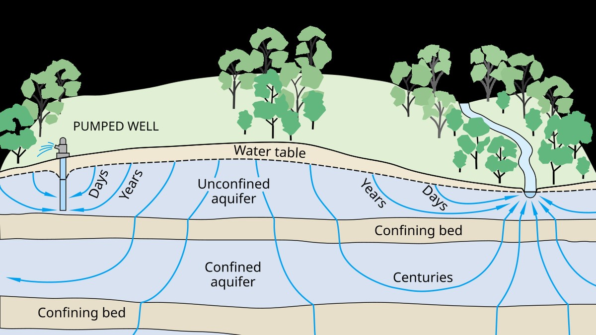
Hydrogeologists classify groundwater storage systems into distinct structural typologies based on geological boundary conditions, stratigraphy, and pressure regimes. The two primary categories are unconfined aquifers (water table aquifers) and confined aquifers (artesian aquifers).
An unconfined aquifer is bounded at its base by an impermeable geological stratum (aquiclude), but is open to the atmosphere at its upper boundary. The upper boundary is defined by the phreatic surface (water table), where porewater pressure exactly equals atmospheric pressure. In an unconfined aquifer, water storage and release are governed by specific yield (S_y)—the volume of water released from storage per unit surface area per unit decline in water table height through physical gravity drainage of pore spaces (typically S_y ≈ 0.10 to 0.30). Unconfined aquifers respond rapidly to local meteorological precipitation, but are acutely susceptible to direct contamination from agricultural pesticides, synthetic fertilizers, and industrial surface spills.
Conversely, a confined aquifer is sandwiched between two impermeable confining geological layers (such as marine clay beds or dense shales) that prevent vertical water exchange. The water within a confined aquifer is under continuous hydrostatic pressure. If a borehole penetrates a confined aquifer, water rises above the upper confining bed to an elevation reflecting the hydrostatic pressure—a theoretical surface termed the potentiometric surface (piezometric surface). If the potentiometric surface rises above the terrestrial ground elevation, water flows freely out of the borehole without pumping, creating a flowing artesian well.
Water release in confined aquifers is governed by the storativity (S) or storage coefficient, which depends not on gravity drainage, but on the elastic compressibility of the mineral skeleton and the physical compressibility of the water itself: S = S_s · b, where S_s is specific storage and b is aquifer thickness. Because water and rock compressibilities are minute, storativity in confined aquifers is orders of magnitude smaller than specific yield (typically S ≈ 10^-5 to 10^-3). Consequently, extracting modest volumes of groundwater from a confined aquifer causes dramatic, regional declines in potentiometric head that can propagate outward for tens of kilometers within days.
Secondary Porosity and Fractured Karst Aquifers
In crystalline rocks (granites, basalts) and dense carbonate rocks, primary pore spaces between mineral grains are negligible. Groundwater movement relies entirely on secondary porosity: structural joints, faults, cooling fractures, and dissolution cavities. In karst terrains, weakly acidic groundwater (enriched with carbonic acid, H2CO3) chemically dissolves limestone along bedding planes, creating subterranean cave networks and conduits. In these systems, Darcy’s laminar flow equations break down; groundwater flows through subterranean rivers as turbulent, high-velocity conduits capable of transporting contaminants miles in hours with zero natural soil filtration.
💧 Geotechnical Hazard: Land Subsidence from Aquifer Depletion
Over-pumping confined aquifers depressurizes pore fluids, transferring overburden stress onto the compressible clay mineral skeleton (effective stress principle: sigma’ = sigma – u). In California’s San Joaquin Valley and Jakarta, dewatering has caused catastrophic irreversible compaction of interbedded aquitards, causing ground subsidence exceeding 9 meters.
4. Baseflow Mechanics and Hydrograph Separation Techniques
A hydrograph recorded at a river gauging station displays the continuous temporal response of stream discharge to precipitation events. Hydrologists partition total stream discharge into two distinct components: quickflow (direct runoff) and baseflow. While quickflow comprises Hortonian overland flow and rapid interflow that produces the storm peak, baseflow represents the sustained, reliable baseline discharge of a river between rainstorms, sustained entirely by subterranean groundwater exfiltration.
The geological interface between groundwater and surface water is characterized by two hydraulic interactions:
- Gaining Streams (Effluent Streams): The regional water table elevation is higher than the stream stage elevation. Groundwater discharges continuously into the river channel across the streambed hyporheic zone, sustaining baseflow throughout dry summer seasons. Most perennial rivers in humid temperate and tropical climates are gaining streams.
- Losing Streams (Influent Streams): The stream stage elevation is higher than the regional water table. River water leaks downward through the streambed into the underlying aquifer, recharging groundwater while losing surface discharge. Losing streams are ubiquitous in arid and semi-arid climates, often drying up completely downstream.
To quantify the proportion of total river discharge supplied by groundwater, hydrologists utilize hydrograph separation techniques. Classical graphical separation methods analyze the master hydrograph recession curve during extended dry spells, which conforms to the Maillet exponential decay model: Q_t = Q_0 · e^(-alpha · t), where Q_t is discharge at time t, Q_0 is initial discharge, and alpha is the baseflow recession constant (typically 0.001 to 0.05 day^-1 depending on aquifer transmissivity and basin storage).
In modern isotope hydrogeology, graphical methods have been validated and refined through geochemical end-member mixing analysis (EMMA). By measuring conservative environmental tracers—specifically stable isotopes of water (Oxygen-18, δ18O, and Deuterium, δ2H) and electrical conductivity—hydrologists can separate the hydrograph into ‘new water’ (event rain) and ‘old water’ (pre-event groundwater stored in the catchment). Isotopic hydrograph separations have revealed a startling scientific truth: in many forested, humid catchments, over 60% to 85% of peak storm hydrograph volume consists not of fresh rain running overland, but of pre-event groundwater pressurized and pushed out into the stream channel via subsurface displacement mechanisms (transmissivity feedback and piston flow).
5. Contaminant Hydrogeology: Advection, Dispersion, and Retardation
The transport of anthropogenic pollutants through subsurface aquifers threatens global freshwater security. Once a chemical contaminant—such as agricultural nitrate (NO3⁻), industrial chlorinated solvents (trichloroethylene, TCE), petroleum hydrocarbons (benzene, toluene), or heavy metals—infiltrates the water table, its migration is governed by the advection-dispersion-reaction equation (ADRE).
Advection: The transport of dissolved solutes carried passively along by the bulk velocity of flowing groundwater: v_x = q / n_e = (-K / n_e) · (dh / dl), where v_x is average linear porewater velocity and n_e is effective porosity. Because effective porosity is always less than total porosity, groundwater solutes travel significantly faster than Darcy flux indicates.
Hydrodynamic Dispersion: As a contaminant plume migrates, it spreads out longitudinally and transversely, diluting concentrations while expanding its spatial footprint. Dispersion combines molecular diffusion (Brownian motion driven by concentration gradients) and mechanical dispersion (microscopic velocity variations caused by pore-size heterogeneity, tortuous flow paths, and friction along pore walls).
Sorption and Retardation: Many organic solutes and heavy metal cations do not travel at the same velocity as groundwater; they are electrostatically adsorbed onto clay mineral surfaces or partition into solid soil organic carbon. This chemical retention is parameterized by the retardation factor (R): R = 1 + (rho_b / n) · K_d, where rho_b is soil bulk density, n is porosity, and K_d is the equilibrium distribution coefficient. A solute with R = 5 moves through the aquifer at only one-fifth the velocity of groundwater, creating a persistent, long-term legacy contamination plume that can contaminate drinking water wells for decades.
6. Sustainable Yield, Aquifer Depletion, and Managed Aquifer Recharge (MAR)
For over a century, groundwater management operated under the flawed concept of ‘safe yield’—the erroneous assumption that groundwater pumping is sustainable as long as pumping rate does not exceed mean annual natural recharge. As hydrogeologist C.V. Theis conclusively demonstrated in 1940, all pumped groundwater must come from three sources: increased recharge, decreased natural discharge (drying up springs, wetlands, and gaining streams), or depletion of internal aquifer storage. Pumping equal to natural recharge eventually desiccates all dependent surface ecosystems.
Modern hydrogeology operates under the principle of sustainable yield: the volume of groundwater that can be withdrawn over the long term without causing unacceptable ecological, environmental, or socioeconomic consequences—specifically preventing baseflow depletions in salmonid streams, land subsidence, and saltwater intrusion along coastal margins.
To combat regional groundwater depletion, water managers increasingly deploy Managed Aquifer Recharge (MAR) techniques. MAR involves the intentional diversion of excess wet-season surface runoff, treated municipal recycled water, or agricultural irrigation tailwater into subsurface aquifers. Common MAR engineering methods include large-scale surface infiltration basins, riverbed spreading grounds, aquifer storage and recovery (ASR) dual-injection wells, and agricultural aquifer recharge (Ag-MAR), where dormant winter crop fields are flooded to infiltrate water through the soil column.
By transforming subsurface aquifers into active, underground water banks, society can store monumental volumes of water during flood years without the catastrophic evaporative losses, ecological devastation, and high capital costs associated with building massive surface concrete reservoirs, ensuring climate resilience and baseflow security for future generations.